Chromalyzer Product Manual
Main Screen
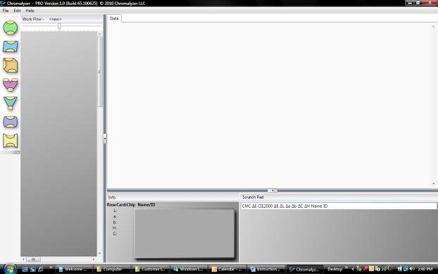
The main screen is divided into two sections the workflow section on the left and the large data view section on the right. In the workflow section you will place elements which represent collections of colors, operations on collections, and various views. In the data view section you will be able to explore these data, functions and views. The size of each of these sections can be adjusted by dragging the edge of the window to shrink or expand the box or by clicking on the  arrow.
The Workflow Section

In the workflow section you will place and link elements.
Each type of element has a different shape Icon and each element has tabs or nodes that you can use to link it to other elements. Nodes on the top of an element are input nodes while nodes at the bottom of an element are output nodes.
To place an element, left click the desired element shape (the element will be highlighted as the active element) and place the element by left clicking again where you want to place the element in the workflow area.
Note: Position all your elements in the location that you want them to appear based on the logical flow of the analysis that you wish to perform.To connect any two elements, click on the yellow output node of one element (at the bottom) then click the yellow input node (at the top) of another element to connect them. Nodes must be connected from output to input. In other words a node at the bottom of one element should only be connected to the node at the top of another.


Double click on the Circle shape in the centre of the connecting arrow to temporarily break the connection between two elements. This is useful when trying to compare the affect of adding or subtracting data to a view. To delete or move a connection, point to the connecting arrow to Highlight the connection and right click to display the Delete or Display option.
Once elements are placed in the workflow they can be moved by clicking and dragging them to the new desired location in the workflow area. You can right click on an element to see other options including the option to delete the element. To rename an element click on its name and use the keyboard to enter a new name.
Elements

The collection element represents a collection or palette of color data. Once you have positioned a data element in the workflow, you can begin by importing existing data.
Importing color palettes

To import color data into a collection right click on the collection element in the workflow area and choose import. Imported files must be tab delimited .txt files, like those created by excel. Selecting the Import file option enables you to locate the file you wish to import using the windows navigate function.
Included with the program are some sample files, in the following example the 1344 Space data file has been imported. You can use this data to experiment with the program.
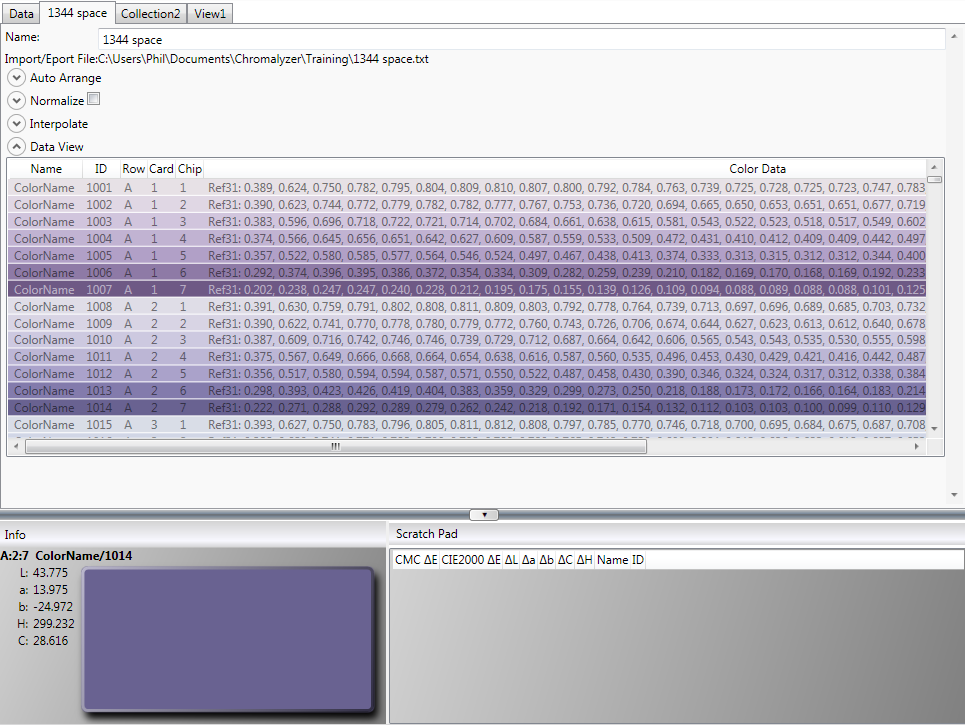
When a collection element is placed in the workflow area a new tab will appear in the data view area with the File name of the imported data file. To view the data that has been imported, double click on the data element in the workflow or left click on the Tab in the data view. Click the Data View  to expand the data window or Click
  to collapse it again.
Moving the mouse over the colors in the data view section will show some of the information in the info area at the bottom of the screen along with a larger sample of the color in RGB form. The area to the right of the Info box is the “Scratchpad”. The scratchpad is a temporary part of the workspace where you can move or copy colors from the main dataset to adjust, manipulate or analyze. It has many uses that we will explore later on but colors can be sent to the scratchpad area by right clicking on them in the list as it is displayed in the main data view window and choosing “Add” to scratchpad. Depending on the type of View sometimes you have the option to “Add” or “Move” a color to the scratchpad. “Add” makes a copy of the color and leaves the original color in the data view, if “Move” color is used the color is removed from the current dataset in the data view and placed in the scratchpad. For now we will just deal with the “Add” data option. When you place colors in the Scratchpad area, as you move the mouse over colors in the list you will not only see information about the color that you are pointing at appear in the info area, but you will also see color difference information displayed in the scratchpad area. This information is describing the calculated numerical difference between the color you are pointing at and all the colors that you placed in the scratchpad.
Note: The method for measuring and describing the differences between any two specific colors is a complex subject with a great deal of material available on the web to explain the metric in detail. The simple concept is that 1 unit of color difference described as 1 delta E (∆E). This is theoretically the distance in “Lab color space” between any two colors that describes a change that is visually perceptible to the average human observer. http://en.wikipedia.org/wiki/Lab_color_space.Importing Data
In order to Import your own data, the format of the data file needs to be quite specific. The format required by Chromalyzer is a tab delimited text file (.txt file extension). There are a number of fields that must be included with very specific “field names” which should include color information in one of several standard formats.
Chromalyzer will recognize color data either as Reflectance, Xyz, Lab, or RGB. Each data field must be tab delimited and these will require a field label that specifies accurately what type of color information in contained in each field.
One easy method to format your color data in a tab delimited text file would be to use a Spreadsheet program. The label at the top of a spreadsheet column is the “Field Name”. The information in the cells beneath the column name (Field name) is the Data.
You can include more than one type of color data in the information that you import in any one collection. When Chromalyzer encounters multiple data types, it will use the “best available” when choosing how to display, and perform the various analysis that are possible.
The priority is 1) Reflectance, 2) Xyz, 3) Lab, 4) RGB. Note: For most accurate comparison and analysis, the input data should be generated from a common source.
It is vey important to ensure that the Field Names for each set of data conform to the format expected by the Chromalyzer program. The color information is a key component and the program will look for certain specific “Field Names”. It is also important to ensure that these “Field Names” are located in the first row of data; blank lines at the top of the file will cause the file to give load errors.
Example Data and Field Names
| ID | Reflectance |
|---|---|
| 12345 | 38.88, 62.43, 75.00, 78.23, 79.52, 80.38, 80.92, 80.99, 80.70, 80.04, 79.24, 78.39, 76.34, 73.87, 72.50, 72.77, 72.47, 72.33, 74.66, 78.28, 80.65, 81.55, 82.06, 83.10, 84.43, 85.77, 86.56, 86.48, 86.05, 85.75, 85.93 |
In the above example there are just two “Fields”. The first “Field” we have given the description “ID”. The second “Field” has the description “reflectance”. All the data for each of these fields follows in columns below these field names. We are identifying the color with an ID number, this “Field” could just as easily be field name “Name” as the data in this relates to how the color is identified, the user has complete control over all the field names and data types but certain field names have very specific purposes and as such the program will look for a number of key “Field Name” descriptions. If possible all data should include either or both “field names” ID and Name as this information is used in the Info window.
Color Data Types
If your input data is in the form of Reflectance data you must have exactly this description for the column or “Field Name”.
Chromalyzer will recognize 16 point reflectance, 31 point reflectance or 61 point reflectance data between 400 and 700 Nm. All data points must be comma separated and must be contained in a single tab separated cell if viewed in a spreadsheet format.
Note: Do not create separate columns for each of the 16, 31, or 61 points, all data for reflectance should be comma separated values in a single spreadsheet column, See example above. Should the data that you have contain a number of data points other than 16, 31 or 61 points, it is likely that it includes data points beyond 400 to 700 nm range, data from these additional bands should be deleted or load errors will occur. Delete any values outside this range from the file. XYZ| ID | X | Y | Z |
|---|---|---|---|
| 12345 | 34.4217 | 34.38728 | 22.03986 |
XYZ data should have a separate field name for each of the 3 data points. It is not case sensitive but the data should be sequential (the X data should be followed in the field name sequence by the Y field and the Z field).
Lab| ID | L | a | b |
|---|---|---|---|
| 12345 | 91.33 | 8.87 | -4.29 |
Lab data should have a separate Field name for each of the 3 data points. It is not case sensitive but the data should be sequential (the “L” data must be followed in the field name sequence by the “a” field and the “b” field).
RGB| ID | R | G | B |
|---|---|---|---|
| 12345 | 34 | 19 | 56 |
Lab data should have a separate Field name for each of the 3 data points. It is not case sensitive but the data should be sequential (the “L” data must be followed in the field name sequence by the “a” field and the “b” field).
Row, Card, ChipThere are two elements that display color data in a 2 dimensional Grid; these are the “Grid” and “Card View” Elements. Both of these display data in positions relative to each other on an X.Y plane as defined by the references entered into each of these 3 data fields. This replicates how color would be displayed for example in a paint color display, a color fan, color card or any other 2 dimensional palette presentation.
Data for Row, Card and Chip may be alpha or numeric and is case sensitive. Priority for the order is as follows:
| 1 | 2 | 3 | A | a | AA | aa | B | b |
Data with the same row designation will be displayed next to one another on a horizontal plane. The column order that they appear in any row is designated by the value of the data given in the Card field. Data with the same Card value will be displayed in a vertical plane, therefore “Card” may also be considered to be arranging colors in a column or series of columns. Multiple colors may be displayed on the same “Card” and these are described with the data in the “Chip” field. Another way to think of this is as a stripe on a card. The following show examples of the layout that results from various values given to data in Row, Card, and Chip fields.
Additional data may also be included with your input data files that may be relevant to analysis that you want to perform using Chromalyzer. Examples of this would be Formula or Popularity information. All data in all fields can be used in filters that allow subsets of data to be described.
Once you have your data in the correct format in your spreadsheet, use the “save as” feature to save the data as a “Tab delimited text file” and provide an appropriate name for this file. Normally the extension for the file will be created by the program as .TXT
Auto Arrange
The Row, Card, Chip sequence can either be created manually to give grid references to layout the colors for the Grid and Chip views, or this sequence can be generated automatically using the Auto Arrange function available in the Data View by clicking on  .
.
This option organizes the data and assigns row card chip addresses based on the values of the colors in the color data and by assigning the size of the grid and the priorities for each of the axes.
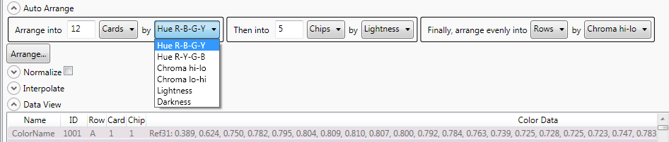
Set the first priority as Rows by Hue, and this will assign the highest priority to the Hue element of the color value, and the flow of the hue will range vertically as evenly as possible from the top row to the bottom row based on how many rows you assign for your grid. Like a vertical rainbow.
You may then set the second priority as being any other value and assign this to one of the other remaining grid references (i.e. Card). Using Chroma Hi-Lo in our example would result in the highest chroma colors in your Range being displayed in the first columns and the lowest chroma colors in the last columns. Our vertical “Rainbow” would now have the brightest colors to the left and the greyest on the right.
Depending on how many colors we are organizing, we can also add an additional dimension to the arrangement and a third priority to the organization. For example if our input data file has 144 colors, if we allocate 6 rows to our grid and divide these 6 rows into 6 cards (columns) each card in each row would automatically be divided into 4 chips (stripes). Each of the color chips on each of the cards could then be assigned a third level priority, for example Lightness would take the lightest of the 4 colors on the card and put this as the first of the 4 color chips at the top, and the darkest on last at the bottom. Arranging the data into 6 rows of 24 cards would cause there to be no third level of priority as there would be just one color per card and therefore no “chips.”
Note: Having set the parameters for the grid size and color priorities or when making a change, click on the “Organize” button to create the new color arrangement. Depending on the number of colors in your file and the speed of your computer this may take some time. The program will display a progress bar to indicate when tasks are running that require extensive calculation.Interpolation
The concept of interpolation is to allow the user the ability to generate new colors with defined equal or variable step values between existing color data points that are “neighbours” in any given grid. Interpolation may be performed to create simple lightness value steps between colors of the same Hue, or create new color Hues between two colors of different Hue, add new Chroma steps between color points of different Chroma, or by providing multiple data points to interpolate between, generate an entire collection of colors where all three factors are taken into consideration.

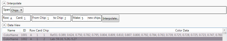
The Following example shows two colors imported into a collection element, and organized to be on the same row and card, in chip position 1 and 2. You could just as easily arrange these side by side as Card 1 and card 2 for a different orientation to interpolate across cards, this example will produce a new set of colors displayed as a set of “Chips.”
To create new colors in between these two colors, click on the Collection name Tab to display the color data and open the Interpolate menu. Select the type of interpolation you want using the Span option to choose between Rows, cards, or chips.

In our example we must select “Chips” and provide detail as to which chips we want to interpolate between. In the event that there are a larger number of rows or cards in your collection you must also give detail as to which row and card the chips are located. Our example is Row A card 1, interpolating 5 new colors between Chip 1 and chip 2.
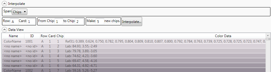
The result is displayed in the data view window. Interpolation will generate color data for the New Colors based on the best data available for the original colors. The Colorimetric data allows you to be able to describe these new colors numerically such that match prediction software used to create products in a wide variety of materials will be able to produce the colors you have generated with a good degree of accuracy to meet expectations.
More Interpolation ExamplesInterpolation across Multiple Chip cards
Original Collection

Interpolate between “cards” 22 & 23

Interpolation Result

Interpolation can also be performed using the Grid element and further instruction can be found in this section.
Displaying Color data in 3D view

The Lab view element is used to view color data in 3D Lab view. Click on the view element on the tool bar and then click this element into the workflow area to create a new view. Connect an output (bottom node) of a collection element in the workflow to the input (top node) of the newly created 3D view. To view the color data in the View, either double click on the View element in the Workflow or click on the view tab in the Display window. In the following example we have imported the 1344 data set provided with the Chromalyzer program into a Collection Element.
Navigating the view

You can rotate the view by clicking and dragging in the 3D view window. The mouse wheel can zoom in and out or you can use the rotate and zoom options in the menu on the right of the screen. Sliders on the left edge and at the base of the window allow you to scroll vertically and horizontally within the view (important as you zoom in and out).
In addition you can change the Pivot point of the 3D display. The default is for the rotation of the display to be around the centre of the color space. If you wish to rotate around one of the colors in the display, point to the color in the display and right click. Select “Centre” from the list of options and this will become the central pivot point for the rotation of all other colors in the display.
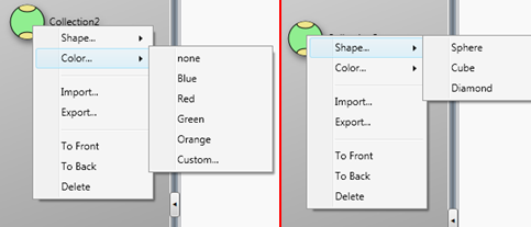
Initially all color data points are displayed as a sphere, and the color of the sphere is the RGB value of the color (either the RGB value imported or converted from the colorimetric data and calculated using SRGB standard). It is possible to change the appearance attributes of the data points in a collection element, which we refer to as the “Tag”. These options are displayed when you point to the collection element and right click. These allow you to change the shape and the “Tag” color.
It is essential to have the ability to change these in order to distinguish between multiple data sets that may be displayed in a single 3D view window for comparison.
The default for the display attributes of the color data tags in a 3d view is for the shape to be shown as it is set in the Workflow window, and for the color to be shown using the color data (RGB). If you want the color of the data points to be shown as the color assigned to the “Tag” you must select this using the menu options in the 3D view window.
These menu options allow you to control the size, shape and colors used to represent the color data within this specific 3D view element. The representative color of the data points in the Display can be chosen from the workflow or the palette. Palette is the default in which each data point has a color that represents the actual color of the sample. Choosing workflow color will change the color of the data points to be the “Tag” color of the collection which you assigned (default color is green).
Note: If no colors appear in the 3D View, check to make sure you have imported or generated color data in the Collection element, and that there are no errors in the naming conventions of the color data fields or errors or unusual characters in the data itself.Adding a second Collection Element and sending this data to the same view allows you to combine the two color collections and see the result of this combination in one view. In the following example we have imported the 144 data also provided with the Chromalyzer program. Setting the 144 element to display as Red and the 1344 element to display as default (green) in the Workflow section creates the following result in the View providing you instruct the view to display color from the Workflow rather than the Palette in the option boxes in the right of the View window.
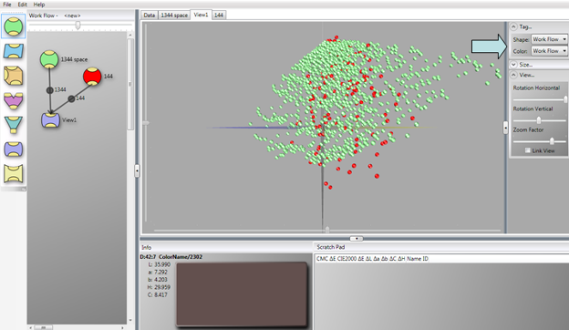
Here we can easily tell which samples are from the 1344 and which are from 144 collections.
The shape of the points can similarly be changed. Experiment with changing how to combine colors and shapes of the color data in the view. The options allow you to display a combination of settings. Informing the view to display shape and color settings using “Workflow” option, shows data points using the form you designate by changing the “Tag” in the workflow settings when you right click on an element and set the workflow display options. Choosing to display Color from the “Palette” option, displays colors as described by the colorimetric data in the collection. Setting the “Shape” option in the 3DView to a specific shape overrides whatever shape you have set in the workflow, and displays all color data points with the shape defined in that 3DView window.
As with all data views, colors in the 3D view may be added to the scratchpad for comparison and manipulation.
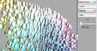
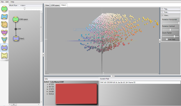
In addition to shape and color you can also control the relative Size of the shape representing the color data points. The calculation for relative size can be set using various industry standard calculations for relative color difference. Here we’ve chosen to show CMC DE ellipsoids at 1.0 radius. Now we can tell easily which samples are close enough to overlap. Colors which overlap when set to less than 1.0 DE according to the standardized color difference equations are considered to be sufficiently similar that the average observer would be unable to distinguish the difference in that aspect of the color variance within the boundary of color space within the sphere. The point at which one color connects at the boundary of another color is the point at which one color becomes visibly different to another color. CMC color space is notable in that each color is represented as an irregular ellipsoid. In general, human observers have a lesser ability to discern variations between lightness and Chroma values for color variation, but are able to discern much smaller variations between colors as they change in Hue. The size of the ellipse also varies in different parts of color space. In practice, these “one size fits all” methods of describing the ability to discern visible color difference are not precise as there are many variables that can not be factored in to these equations, but most industries tend to conform to one or other of these methods for the purpose of establishing some method of common communication and color control.

Multiple 3D views can be set up in the Workflow area. It is possible that you would like to compare the data in some or all of these views from exactly the same perspective when performing your analysis. This can be achieved by placing a check in the “link View” box in the view options.
All 3D views in a workflow which have this option checked will display with the same Zoom and rotation orientation. Making a change in the viewing angle or zoom level in one view will be mirrored in every other linked view as soon as this is displayed.
Exporting Combined Data

Having combined two sets of data in a 3D view, it may be that you need to save the result of this union of data. This can only be achieved by first transferring the data into a new collection element as in the following example.
It is not essential to have the 3DView element in the sequence, simply sending the 1344 space data and the 144 data into a new collection element would allow the union of the two files and enable this to be exported just as easily.
It is likely that the data fields in the two collections that are now joined in the combined collection are identical. It may also be the case that the color data from each is also different i.e. one may have reflectance data the other may be L*a*b format. Simply exporting the data will result in a file that contains a list of the union of the data in all of the combined fields.
However it may be that your preference is to select just some of the fields from the two data sets. It is also possible that there is data in one collection which mirrors data from the other, but it is identified with a different “Field Name” for example the color ID in one data set may be in a field name that is properly described as “ID” however the ID data in the second data file may have the Field Name “Code”. In this case prior to exporting the data, rather than having these two pieces of data in different “Fields” you may prefer to merge these under the same field name. This can be done using the “Normalize” option the data view (displayed when you double click on the new collection element or open the tab in the data view).
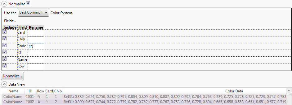
Opening the Normalize tab displays all the field names of the data to be exported. Renaming the field Code to the same name as ID, will cause the data from Code to be merged into the ID field when exported. When “Normalizing” data, this also causes variations in Colorimetric data to be condensed into one common format. The default is “Best Common” which is to say that of all the variations that occur in the combination file, if some data points use Reflectance and some use L*a*b*, all exported data will be in L*a*b*. (L*a*b* can be derived from reflectance but not the other way around). Clicking on “Normalize” generates this integration of data. In order to actually perform the export to save the normalized data as a new collection file, right click on the new collection element and select the “Export” option. Save the file to your computer with a filename of your choice. Chromalyzer will attach a .TXT extension to whatever filename you select. Note: When trying to import a file exported by Chromalyzer using a program such as Excel, remember to set the Open Files option to display File of type “All Files”.
If you want to convert reflectance to L*a*b*, or get RGB from L*a*b* etc, you can also use the “Normalize” function. Change the “Best Common” option to the color space that you prefer. Chromalyzer can calculate required data providing the original data is a higher order to the data type you want to generate.


The Card view icon represents an X,Y Color Chip view of the data just like color chips in a color chip display in a paint store or on a color sample card. The card view uses row, chip and card. Information included in the imported or generated data associated with each sample to arrange them in the card view.
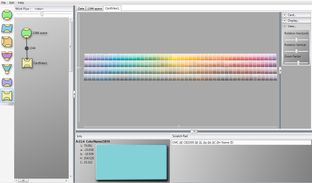
The card view contains several controls to adjust the dimensions of the cards and the display itself. Width and Height adjust each card. Chip margin affects the white space on each card. Card gap represents the space between each card. For the display there is a row overlap control. This adjusts the amount of each card that is occluded by the row in front. Row offset adjusts how far each row is from the row behind. Curve is the total angle of curvature in the display. This display is also able to be rotated in much the same way as the 3D view to allow the over display to be viewed from various angles, when the display is in high zoom, the display may scroll left to right and up and down using the sliders as in the 3D view.

Card view displays chip relationally as they are organized in rows, cards and chips. Any gap in the numbering system of rows and cards will result in a gap in the display in the Card View window.
The exception here is chip. In the Card menu with the “Stretch Chip” option displayed if there are Grid references for row card and chip locations but no color data for these locations there is no blank space displayed, instead the other chips on the card are increased in size equally to fill the entire space available on the card.
Colors interpolated in the Collection data view will be given Row card and chip grid numbers that will immediately appear in the Card View.
More than one collection can be attached to a single Card View. Row card and chip grid references should be unique for each collection to avoid displaying colors in the same location. Card views which have more than one Collection element connected will display all data which has duplicate Row Card and Chip grid references in the same position. Cards and Chips will be divided to accommodate multiple colors.
Info Box and Scratchpad
Information about specific samples is displayed in the Info box as you move the cursor around the data view, 3D view or the Grid and Card Views. This includes Row, Card and Chip information if entered, (Row A, card 3, chip 2 in this example) as well as displaying the Name and ID. If there are no fields entered as Name and ID, the info box will assume the first two fields of information imported are Name and ID and will display this data as Name and ID.

Right clicking on a sample while pointing to the color in any display view will give the option to send the color information for this color to the scratchpad area. It is possible to send multiple colors to the scratchpad area to create a subset of colors that you want to analyze. As you move the cursor over other colors, either in the View display or in the scratchpad area itself these colors will become highlighted. The differences between the highlighted color, and all the other colors in the Scratchpad are described in “Delta” color difference values in the scratchpad data box.
It is possible to Export the list of colors complete with all color data from the scratchpad to create a new unique collection, or to import colors into the scratchpad. Left click on the word “scratchpad” to select these options
Editing Data Points
It is possible to edit the data imported into a collection when displayed in most views. It is important to understand how the program handles these changes and how and when these changes will become permanent changes to your original stored data.
When color is imported into a collection element, this data can be displayed in the data view. Pointing to this data and right clicking displays an option to edit data. Depending on what format the original color data was provided, you will have the option to make adjustments to the actual color values in any appropriate calculable “Space”. If your raw data was Reflectance, as this is the highest order of color data you will be able to adjust the color values using reflectance, if the initial input data did not include this data it is not possible to accurately synthesize these values therefore you will only have the option to use that space or “Lower order” spaces.
Note: Data imported as reflectance and Edited using a lower order color space Model such as L*a*b will result in Reflectance data for that revised color sample to be unavailable.As you make changes to the color data in the imported collection, they will be reflected in the color displayed in the current view, and any other view that this data is connected to in the workflow. I.e. if you have a 3Dview element connected to the Collection element, the relative location of the color data point will be adjusted when you next open this view. However the original data file that you used to import this data remains unchanged. If you wish to permanently change the input data file, you must “export” the data from the collection element in which you have made the changes, and either create a new file that will include these changes, or overwrite the existing file that you originally imported by saving the new data with the same name as the existing file.
It is also possible to change data for colors that are copied to the Scratchpad. Pointing to a color in the scratchpad and editing this color data, does not affect the data of the color in the “collection Element” or in the original imported data file. You have in effect made a carbon copy of the original color and this is being held in the Scratchpad. Any changes made in the scratchpad are to the copy only. Again it is possible to permanently record these changes by exporting this data to a new data file.
If you wish to replace the data of a data point in the “collection” with that of the edited data of a data point copied into the scratchpad, this can be achieved by replacing the original matching data point in the original “collection” File with the edited color data from the scratchpad using the export option using Excel or other file editor. Alternately you can manually edit the original color in the Collection element and copy the data from the scratchpad version.
Filters

The filter elements allow you to filter the data in a collection based on a set of criterion that may be specified by the user about each data point to limit the number of samples in the output.
Filters may be set to specifically include or exclude individual colors or groups of color data and create a sub set of the data that has previously been generated or imported into a Palette. Filters can be set to analyze data points based on either the color values, or on the other user defined fields in the data records.
Data can be considered to fall into one of several categories.
Text or Alphanumeric:Any combination of text, characters or numbers in a field i.e.:


Colorimetric data can be filtered based on either individual numeric data in each field or based on the relativity of the color values as defined by the color data i.e. Hue, Chroma and Saturation.
Place a Filter Element into the workflow area between the Collection Element and View Element. Connect the output node of the collection to the input node of the Filter Element.

Connect the output node of the Filter Element into the input node of the View element.
Double click on the Filter element or click on the Data tab and open the filter to display the settings.
Choose the type of filter from the list of available options and set the parameters required. In the case of filters based on Color Attributes the choices are filter by Hue, Lightness, Chroma Band and Reduction.

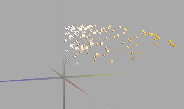
In each case, a To and From value should be entered to describe the range for the criterion of color that should be met. Only colors that fall within this range will be passed through the filter. Multiple filters may be set to establish several criterion that the data must meet. Also more than one set of data may be passed through the same filter. In this way it is possible to find for example all colors from two different collections that fall within a specific Hue angle range and are within a lightness range from level 61 to 90. The following is an example of this data displayed in a 3D view. One set of data are shown as Squares the other as Spheres.
Reduction
The reduction filter may also be referred to as popular reduction. The principle behind this filter is to reduce the overall number of colors to a smaller set based on where colors are clustered. Selecting this option requires you to select additional settings
“Color Space” option allows you to select the model for the relationship between colors and defaults to Lab. You must also set the number of colors that you want the collections to be reduced to. This can either be a % of the total or can be set to a specific number.
Reduction by Volume performs analysis by first dividing the overall gamut of the color space into an even number of regions and finding the centre of popularity in each region. By density reduces the number based on clusters of color as a percentage of the overall total irrespective of overall coverage.
The following shows an example of the outcome of reducing the 1344 palette to 20 based on volume compared to density.

Custom Filters
Custom filters allow all data fields to be searched based on a set of functions and logical operators being applied to the data in that field in each collection.

The field name should be typed in the box between the [] brackets for example [ID] selects the data in the ID field for the filter analysis. Open the tab in the middle to display the range of Functions and logical operators for the type of analysis to be used in the filter. Finally select what criterion should be met in order for the filter to include or exclude data passing through the filter. For example a custom filter that uses [ID] .contains. “B15” would assume that there was a “Field Name” heading of ID, and would search every data point passing through the filter who’s ID included B15. All records with this ID would pass, all others would be excluded.
The syntax required for these functions is as follows.
.Equals. Exact criterion must be met. Example [ID] .Equals. B15 would select a data point with B15 in the ID but not a data point with the ID B151
.Not Equal. Opposite of Equals.
.Less Than. Requires Numeric data. Example [ID] .Less than. 20 includes all data points with an ID value below 20 It would not include B19 as this contains alphanumeric data and is therefore not able to be analyzed as a simple number. -19 would be included as this is a negative number.
.Less than or equal to. As above but the number 20 would also pass, which it would not in the case of .Less than.
.Greater Than. Requires Numeric data. Example [ID] .Greater Than. 20 includes all data points with an ID value above 20 but would not include B21.
.Greater than or Equal to. As above but the number 20 would also pass, which it would not in the case of .Greater than.
.Comes Before. Similar to Less than but works with Alpha Characters. Example [Name] .Comes Before. “Butter” would include names where the first word started with alpha letters before these. “Beautiful Green” for example would pass the filter, “Byte” would not.
.Comes After. Opposite of comes before
.Is or Comes Before. Includes words before and those containing the exact letters in the reference.
.Is or Comes After. Includes words after and those containing the exact letters in the reference.
.Contains. Any part of the string of alphanumeric data should be present.
The .CONTAINS. function is very powerful. There are some special characters you can use to search for various patterns. For example:
[Name] .CONTAINS. ("gr[ae]y") will search for things with "grey" or "gray" in them. the [] means any of these characters. You can also give it a range like [a-z] or [0-9].
[Name] .CONTAINS. ("blue$") looks for things that end in "blue". (This is how .ENDS WITH. works.)
[Name] .CONTAINS. ("^blue") looks for things that start with "blue". (This is how .STARTS WITH. works.)
[Name] .CONTAINS. ("blue|green") looks for things that have "blue" or "green" in them. The | is and or. (notice there are no spaces, if there were it would search for those too which may not be right.)
[Name] .CONTAINS. ("ous(\\s|$)") looks for words that end in "ous". Here the ( ) are groupings, the \\s mean any white space and again the $ is the end of the line. So it looks for "ous" followed by either a space or it is at the end. We code have also just left a space " " in for the \\s since usually the white space will be a single space in our data, but \\s is more correct.
[Name] .CONTAINS. ("[aeiou]{3}") will find everything that has 3 vowels in a row. The {n} means n of the thing before, which in this case is a [ ] grouping meaning any of these. You can also give it a range like {2,3} meaning two or three of the thing before or {2,} for 2 or more. There is also the short hand + meaning 1 or more and * meaning 0 or more.
[Name] .CONTAINS. ("(\\s|^)\\w{3}(\\s|$)") uses \\w meaning any word character (i.e. letters) to find all the names that have 3 letter words in them. So, find a space or the beginning, then 3 letters then another space or the end. There is also a \\d that means any digit.
Be careful when using \\s, \\w, and \\d that they are lower case, the upper case versions mean the opposite like \\S is any non space character and \\D is any non-digit character.
A full list of all the possibilities is available at the following web site:
http://msdn.microsoft.com/en-us/library/az24scfc.aspx
.Does Not Contain. Opposite of above.
.Starts With. Any string of characters at the beginning of the specified field. Example [Name] .Starts with. “Terr” would include Terra Firma and TerraCotta.
.Does Not Start With. Any string of characters not at the beginning of the specified field.
.Ends With. Include all records with the reference string at the end of the field.
.Does Not End With. Include all records without the reference string at the end of the field.
Advanced allows you to construct your own range of custom filters and include additional constructs including and or xor statements.
Grid Element

The grid element is in some ways similar to the Card View in that it requires data to have Row Card and Chip grid references in order to display color information, however it provides many more functions to edit and manipulate the organization of the collections that are input to a grid element.

Clicking on the Input colors opens a window to display the input data in the same format as the data view of a collection element.

You can use the grid with this data window open or closed, but this offers a useful snapshot of the data that can also be displayed in an XY plane in the “Grid” view.
When data is sent to the grid initially it is not fully displayed in the Grid view, this is deliberate as drawing the grid can take some time based on the number of colors that are in the collection. Any changes made to the data flowing into the Grid are not made automatically as this would slow the program down significantly if the grid were to be redrawn automatically each time any of a series of prospective changes were made, i.e. adding a series of new filters. The initial input of data collections, and any changes to the input that would affect the display must be redisplayed with a manual instruction to “Create Grid” by clicking on this option. A message next to the “Create grid” option alerts you when changes have been made to the input that is not currently being displayed.
Selecting “Create grid” displays the color cards/chips in the data view; these can be temporarily hidden or displayed using the toggle option.
The slider zooms in and out to show larger samples or more colors in the grid. Drawing and manipulating colors in the grid view is very processor intensive. Displaying more colors in the Grid view increases the demand on the processor and you may notice some delays displaying large grids.

Scroll bars to the right and at the bottom of the screen allow you to scroll through the entire display when using Zoom. Cards can be displayed in Vertical or Horizontal orientation, (Changing this option will not display until Create grid is also selected).

More than one collection may be sent to one Grid element. In the event that the Row Card and Chip data in these files is identical you have several options.
In the following examples we will merge two sets of data that have the same Row Card and Chip data, displayed stand alone they each look as follows:
1344 colors 144 colors

Sending both sets of data to the same “grid” causes conflict with which database retains the existing “row card chip” data, and what new “row card chip” values should be assigned to the newly added data.

With the Inputs Only option selected, any changes that may have been made to colors in the existing “grid view” will be overwritten by the data from any and all collections that are attached to the input node. The “Row Merge Method” option determines how the data will be combined. The Default option is “append rows”. This causes the data that was most recently added to the Grid to be given row values that are sequentially higher than the existing data in the grid.
 Interleave Rows

Adds additional data with duplicated data inserted between existing rows.
 Merge Rows

In order to "Merge" data into the rows, an additional option must be selected to determine how to merge the cards that have duplicated values. The default option is to Append, which places the most recently added data behind the cards that exist in the grid.
 Interleave Cards

Interleave insets the cards in between existing cards in the grid
 Merge Cards

All card numbers that are duplicated retain the same value; the added data is merged as additional chips on each card
 Merge Existing With Input

In many cases the original data that was sent to a Grid element will have been modified, as in the example below where cards have been moved from their original location.

The Row card and chip data in the “Grid” is now different from the original data in the “collection” element that is connected to the “Grid” element. Adding new data to this grid and selecting “Create Grid” with the “Inputs Only” option set will cause any changes that are made in the grid to be lost. The grid will be redrawn with all the original data from the collection elements
Note: A message will warn you when this option may cause data to be lost, this is normal.In order to retain any changes that have been made so far in the grid, this option must be changed to “Merge existing with Inputs”. In this case the new data will be inserted with the Row Card Chip values as they currently appear in the grid
 IMPORTANT NOTE: When merging a new or additional data collection element into a grid where changes have been made that you wish to retain, remember to disconnect the collection that provided the original data. Failing to disconnect this data collection element will result in that data also being added back into the grid. Effectively you will have 3 sets of data in the grid, the original adjusted data, the added data, plus to original data re-imported (see below)
 Add Blank Grid

This option allows you to create Blank rows columns and Chips according to the format criterion that you set.
It is possible to retain the changes made to a grid as well as displaying the original data from a collection. To achieve this you must send the output from your edited grid into a new grid that also has the original data as a combined input. Selecting “create” on this new grid will allow you to combine the two sets of data according to whatever merge settings are preferred.
Note: When editing data in the Grid element it is not possible to edit the Row Card Chip fields. These are permanently linked to the original input data. When you move a color using any of the tools that enable this to a new location, the Row Card Chip data is altered automatically. IN order to save this data permanently, a new collection element must be linked to the Grid and data may be exported from here. IMPORTANT NOTE: In the event that you make a mistake with these merges, don’t panic, the Undo option will restore you to the point you were at immediately before this action was taken. However as these merges can involve a significant amount of time to calculate, and especially if a significant amount of work would be lost in the event of any problems, it is strongly advised that you “save” your project before performing the Merge.Nesting Grid Elements

One tip that may help you not lose any changes that you have made to data in your grid when you start merging additional collections is to direct the data from one grid directly into another grid. Each time you use the “Create” button to redraw a grid, it will only affect the data in the one grid that you select for this action. I.e. if you send data from grid one to grid two, and “create” grid 2, you now have tow identical displays. If you add more data to grid 1 and “create” grid one to redraw this grid, grid 2 remains as it is, only grid one has changed. In this way you can have multiple versions of any given layout accessible at one time.
Moving colors in the Grid
There are several options available to manipulate either entire rows of color data, or entire columns of cards, as well as options to manipulate individual cards and or chips on the cards. By pointing to a Row or Column label and right clicking, these options are displayed.
Rename/Move/Swap Row prompts you to enter a new “Name” for this row. If you currently have Four rows (A,B,C,D) Renaming row A with the letter E will cause Row B to become the first row and the renamed Row E to be displayed as the last row. Renaming Row A as Row C will cause these two Rows to swap names and places. Rows may be given complete names i.e. “Clean Colors” or “Muted Colors”. The order that they are displayed is dependant on the alphanumeric order described previously.
Insert Row creates a new row of blank chips beneath the row. This row is given a row number consistent with the current order i.e. inserting between Row A and B will result in the new row becoming Row B. If you wish to insert a new row above Row A create the new row below Row A and use Swap Row.
Populate Row will give you the option to define the number of Chips on each card across the row. Initially these chips will have no color values. Populate Row will have no effect on a row that already contains chips.
Interpolate Row creates a new row of color derived from the colors in the cards/chips of the rows above and the rows below the new row. In the event that there is a difference in the number of chips on each row, the interpolated row will contain the lower number of chips and the interpolation for each color will be calculated as being exactly 50% in-between the color values of the chips of equivalent chip number of the interpolated rows.
Creating more than one New Row between existing rows, and selecting “interpolate” on any of these new rows will create new colors in all of the Blank Rows using the data from currently populated rows above and below. In this way you can create rows of new colors that have variable Step values of interpolation. I.e. if you wish to create new colors that are 1/3rd steps between existing colors, create 2 new Rows, if you want 25% step values create 3 new Rows. This principle is consistent throughout all Interpolation options for Rows, Columns, Card, and Chip interpolation.

The actual color values created will be derived from the “Best Available” data for each of the colors used in the interpolation.
Note: the principle of Interpolation is also described in the section on Data View.Clear Row Chips, removes the color data from all the chips in the selected Row leaving the blank chips in place.
Clear Row Cards/Remove chips. Leaves the Cards in the Row but completely removes all the chips from the card. This basically creates a blank row or gap in the overall color grid.
Delete Row completely removes the Row from the Grid. Removing a Row does not result in the automatic renaming of the remaining Rows to follow the new sequence.
Manipulating ColumnsPointing at any of the Column Headers (Large box at the top of the column containing the letter or number identifying the Column) in the grid and right clicking displays options similar to the Row options to manipulate all the cards and chips in that specific Column of color.

Insert Column (before and after) creates a new column of cards in each Row without chips or color data either in front of or behind the selected column. The Column Number for the cards in the inserted column adopts the value for a new column in the logical sequence and all other cards are shifted to subsequent columns. The “Card” value for the data in the color remains the same as the original imported data until it is exported to a new collection .TXT file at which time it is assigned a Row Card and Chip value that is pertinent to the relative grid location.
Rotate Column To Front. This option allows you to select any column and have this become the first column in the sequence. All other columns remain in the same logical order. Imagine the columns are on a circular turntable, all of the columns to the left of the column that is selected to become the first column are moved in the same order and are added to the back of the list.


As described above Row Card Chip data is altered in the chip Info to reflect the latest location but unchanged in the “Input Data Collection” for the colors in the grid display. Changes only become permanent once exported to a new file or overwritten and saved with the original file name. This is consistent when any color is placed in a new location using any method.
Interpolate Column. Works exactly as Interpolate Row except creating new colors in between Columns
Clear Column Chips, removes the color data from all the chips in the selected column leaving the blank chips in place.
Clear Column Cards/Remove chips. Leaves the Cards in the column but completely removes all the chips from the card. This basically creates a blank column or gap in the overall color grid.
Delete Column completely removes the Column from the Grid.
Manipulating Cards

The location of a card can be swapped with any other card by Dragging and Dropping a card to new location. Point to the card header (Area at the top of the card containing the letter or number identifying the Card) left click and hold the button down while you move the card to a new location.
Pointing to the header of a card and right clicking displays the options to manipulate Cards
Insert Chip (top) creates a new Blank color chip space in the first location on a card; Insert Chip Bottom places a blank chip space as the last chip.
Insert Card (left) adds a new card just in the same row as the selected card. This new card has no chips. Insert Card (Right) places the blank card to the right of the selected card.
Rotate card to the front has the same result as Rotating the entire Column except only the cards in the same row are rotated.
Reverse chips takes the color sequence from top to bottom and completely reverses them for just this card.
Interpolate (across) requires a new blank card (or set of cards) to first be inserted between cards that contain color data. Interpolate (down) interpolates using the color or colors in the cards above and below the blank card (or cards) to receive the interpolated colors.
Clear Chips, deletes color data leaving blank chips on the card, Clear Card/Remove chips leaves a completely blank card in that Row and Column, delete card removes the card completely.
Manipulate ChipsThe location of an individual color “Chip” in a grid is most easily changed by “Dragging and Dropping”. Point to the color you want to move, left click and hold the left button down while moving the pointer to the new chip location. If there is existing color data in the new location, the two data points will swap places. Holding down the Shift key while dragging and dropping Copies the data from the original location to the new location. If there is existing data in the new location this will be overwritten. You cannot “Move” a color from one card and add the data onto another card using drag and drop. To do this you would need to Move the color to the Scratchpad from one card, select the card you want to add this to, “Insert” a new chip on that card then point to the new chip and select “Move Scratchpad Color Here”. Point to the individual chip and right click to display all the options for manipulating chips.
Insert Chip (above or Below)

Selecting this option allows you to open up a space between existing colors in a card, or on a new blank card. This would allow you simply leave spaces between existing colors, or to input color data into this location, by any of the means possible with Chromalyzer, such as moving colors from the scratchpad, or entering color values into the color data fields or interpolating or extrapolating colors.
In this example, pointing to the top color and selecting Insert chip below opens a space between the first and 3rd colors on a card.
If we point to the blank color chip and right click you can select Move Here from Scratchpad to place any color from the list of colors currently in the scratchpad into this location.
Selecting Interpolate allows will generate new color data for the Blank chip, using the color information from the color above and the color below. Effectively you will have a new color that is exactly 50% between the colors immediately above and below the inserted chip. If you wish to create 2 new colors, insert 2 blank color chips before interpolating, this will give you 2 new colors exactly 1/3 between the colors above and below the spaces on the card.
Extrapolate

Extrapolation allows you to create color data into a blank color chip that is an extension of color values. The default color values used as reference 1 and 2 for extrapolation are the last color on the card, and the color immediately above the blank chip to be extrapolated. A sliding scale determines the multiplication factor of the two color values that is applied to create the new color data.

To choose different colors as the values to be used in the extrapolation, point to the color chip in the Reference #1 or #2 box and Right click, this will allow oyu to clear this chip, repeat the Right click to display the menu again and you can now import any color as the reference chip from the Scratchpad (note: you will first have to place the colors that you want to use for extrapolation into the scratchpad).
View/edit data opens a new window with many additional options

Add User Field allows you to generate an entirely new user defined Field Name and add data into that field for this specific color data point. Editing other color data points subsequent to adding a new field will display this new field and allow you to make entries into this field for other data points as well.
Clicking on any of the Color Space tabs (i.e. LAB, XYZ) enables you to adjust the color values of the color based on the parameters applicable to that space. Again the ability to manipulate color data in each space is dependant on the format of the original imported data. Color can only be adjusted in color spaces equal to or below the highest order of the original data.
Opening a tab and selecting the “define with” option displays Sliders which allow you to vary the appearance of the color, or you can click on the numerical values and key in new data. Accepting this data changes the color values in the Grid display It is not yet saved until sent to a collection and exported to create a new collection, or saved as a Chromalyzer project file.
Note: All changes made to color data in the Grid Element are not permanent until saved as a Chromalyzer Project file for recall by the program or exported as a new collection to a .TXT file.Function Element

The Function element is designed to enable comparison between color data from two or more collections. Color data from one or more collections connected to the left hand node of a Function element may be compared to one or more collections connected to the right hand node.

Double clicking on the Function element or clicking on the appropriate Function in the Data Tab in the Data View window displays a Venn Diagram which is used to set the parameters by which the color data in each of the input data collections will be compared.

Check the Use Comparison box to select the type of DE calculation model preferred to generate comparison information of the data sets.
With the DE comparison set, these diagrams show how you can display only those color points that meet the set criterion. With a 2DE comparison function set for the comparison of two data sets, All colors from the data collections that are entered into the left node (set A) will be compared to all colors from the data collections that are entered into the right node (set B).

The Color Data points from each collection are said to intersect only where the criterion of the function are met.
Clicking on each of the 4 regions of the diagram toggles that region “On and off” to inlude or exclude the data that is calcuated to be matching criterion set for the comparison. In this way numerous permutations as to which colors from each data collection are “Similar” or are “Dissimilar” according to what your criterion is that defines similarity in terms of the DE value you set.
In the above example all colors from Set A (connected to the Left node Function input) that are calculated to be within 2DE of the comparison database Set B will be said to be in the intersection of A+B, and all colors from the Set B (connected to the Right node) that have a color within 2 DE of the comparison database in Set A will also be said to be in the intersection of B+A.
Selcting the Generate Proximity Report allows you to export a full list detailing each of the colors from palette B that fall with the DE range specified for match to palette A. including the DE value of the match.
Using the Venn Diagram it is possible to separate and display these colors from any combination of:
Show only colors from A that meet the criterion
Show only the colors from B that meet the criterion
Show all the colors from A that do not have a color in B that meet the criterion (Vice Versa)
Using this method many varied comparisons can be made
What each shape means…
Full union (all shapes on) will include everything from the left and right. I.e. all colors from both databases including those that are within 2DE of any other color in both original databases.

Include everything on the left that is not also on the right. I.e. subtract right from the left. (A-B) i.e. Just display all the colors from data set A that do not have a similar color from Data Set B that is within 2 DE.

Include everything on the right that is not also on the left. I.e. subtract left from the right. (B-A) i.e. Just display all the colors from data set B that do not have a similar color from Data Set A that is within 2 DE.

Include Colors that are on both the right and the left. I.e. only those colors in Both A and B that are similar (within 2DE)

Include Colors that are from the left and the right but not both (“Exclusive or” or “XOR”) i.e. Colors in Database A and B that are dissimilar (have no other colors in either database within 2DE)

Include Colors on the left that are near at least one Color on the right

Include Colors on the right that are near at least one Color on the left

Include all colors from Database A that have no Similar colors from database B, Plus colors in Database B that have similar colors in Database A. Effectively this replaces Colors in Database A that are similar to colors in Database B with the colors from Database B that are the close matches.

Include all colors from Database B that have no similar colors from database A, plus colors in Database A that have similar colors in Database B. Effectively this replaces Colors in Database B that are similar to colors in Database A with the colors from Database A that are the close matches.
Matrix Element

If you had trouble understanding the Movie, just wait until you try and figure out how to use this feature! However for anyone who is tasked with organizing or reorganizing color palettes, this tool is well worth taking the time to understand.
The key to using the Matrix to arrange your palette, is in comprehending the nature of Color Space, and how Chromalyzer allows you to define the flow of a color palette, and the relationship between colors that are considered to be Adjacent.
It may seem like a simple task when laying out a color palette in a 2 dimensional plane to choose which colors belong side by side. In the spectral rainbow Purple is followed by red, then Orange, Yellow and so on until we get back to Purple. A perfect circle of color. This does not factor in all Nuances of color however.
L*a*b* is a 3 dimensional model for a color space described in terms of lightness, Hue and Saturation.

The LAB view clearly shows where colors sit in relation to one another based on their relative colorimetric values in LAB space. However when laying out color in a one or two dimensional plane, decisions must be made as to which colors are placed adjacent to one another. This requires a priority to be given to each of the 3 planes of the 3D model. More information on definitions and various color space models is available as sites such as http://en.wikipedia.org/wiki/Color_space
Chromalyzer allows you to organize according to lightness values, Hue values and Chroma values. There are many ways to organize colors and priority must be given to one value over another if you wish to take a 3 dimensional model and display it in a 2 dimensional grid. Consider the following example for the arrangement of the exact same set of colors.

The first arrangement above arranges 120 colors such that colors are organized with priority given to similarities in Lightness and Chroma.

The second arrangement uses the exact same set of colors, but priority is given to placing colors of similar Hue adjacent to one another.

The third organization breaks this down still further, creating different priorities for Bands of color where the priority for Hue is broken out for several bands of Chromatic values. The matrix gives you control of how you define the rules for the color space that defines how you wish to arrange your palette, and enables multiple “what if” scenarios to be performed almost instantly.
In order to describe where LAB colors are placed relative to one another in the one or two dimensional, plane the Chromalyzer program allows you to define a Matrix for a color grid using the 3 values, Row Card and Chip and to assign color values for this grid using a cubic representation for what we call the RCC color space.

It is possible to generate new color collections by describing the gamut or boundaries of the colors that are available for you to include in a new palette. This we refer to as your RCC color space and it is this that Chromalyzer will divide into a series of individual matrix colors. However many colors you wish to specify for the new collection will be organized into a matrix of rows cards and chips that is a representation of the overall gamut defined in the RCC color space.

The Matrix Definition scale controls allow you to generate a theoretical gamut of color in the RCC cube and allow you to set a range of color values for each of the 3 matrix parameters. In the RCC Matrix the Card parameter controls the range of color that runs from left to right and is the front elevation of the cube. You can set Start Hue, How Light the initial color is and how saturated. If you were to divide the RCC space into just 7 Cards, the end result would be that you would have 7 colors that were each the average or most central point of each of the seven Matrix Zones that the RCC cube was divided into across the face of the RCC space cube.

If we wish to divide this RCC space into a series of cards with more than one row of color cards, we must describe in what way the subsequent colors chips should vary from the initial color on the card for each of the extra rows we are going to add. By changing the Parameters of the Saturation, Whiteness and Blackness for the Rows you can establish the gamut for the range of color variation that will be apparent between each Row of colors that are eventually created in the new palette.

The variation between the level of Whiteness, Blackness and Saturation between the settings you choose for Card and Row will become apparent in the color from the top of the RCC cube space to the color at the bottom of the space.
If we wish to create 2 rows of 7 color cards in our new collection the resulting 14 color samples will be the average of the color values described by the 14 matrix quadrants for the colors in the face of the RCC cube.

The colors in the first row have been set to be lighter than the colors in the second row, but they will still share the same basic Hue.
We can also add additional color Chips to each of the 14 color cards effectively creating let downs or stripe cards for each card in each row. Again the difference between the levels that are set for Saturation, Whiteness and Blackness between the levels for the card and the levels for the Chip will determine the gamut and the range of difference between each of the chips that we want to add to our new palette. If we want to add just 3 chips to each the 7 cards on each of the 2 rows, we are now creating now 42 Matrix quadrants that will be averaged to create the 42 colors in the new palette.

Having used Matrix Definition controls to define the gamut it is now possible to key in the values to generate the colors for the Rows, Cards and Chips

The Generate New Color If No Match option should always be checked if colors are being generated from theoretical color space defined by the Matrix color scales. All other checkboxes should be left blank as they are not relevant when using Matrix defined RCC color space. Key in the number of Rows Columns and Chips you wish to generate and the Generate option will create colors according to the defined settings. Send this output either to a Card View or a Grid to display the results.
 Using the Matrix to arrange Measured or Real color data
In addition to Chromalyzer generating colors for each Row Card and Chip location that correspond to the RCC color space as defined by the Matrix Definitions, it is possible to allocate “actual” colors that match to the generated color values.
The Data to be used by the Matrix element should first be imported into a Data Element, and then connected to the input element at the top of the Matrix Element.

The definition of how close this match has to be in order for the Matrix to use this color rather than create a brand new value is defined by the “Limit Matches To" Tolerance of” box. Make sure there is a check in the box indicating that this feature should be activated.
Selecting this option and limiting the matches to 5 DE for example, causes the program to first calculate what the optimum color values would be to create a collection of colors that conforms to the gamut and RCC arrangement specified by the Matrix definitions. It will then compare each of these color values to all of the colors in the Input Database. Where there is a color value that is a “match” between the calculated color and any given color in the input data file, instead of using the Generated color value for this Row Card or Chip location the color from the Input data file will be used instead.
In some cases based on how loose the tolerance is that defines a match between the calculated Matrix Grid color value and the color values in the input database, there may be more than one color in your input data file that is a match for any given Row Card and Chip grid location. Also you may find that some colors in the input database could be a match for more than one of the Matrix defined RCC grid locations. In this case you have several options.
Checking the box “Use each color only once” will result in each color in the input data file being assigned to the grid location where it is the best possible match and not being used again.
Checking the Box Limit to one color chip per location will prevent more than one color from being placed in the grid location of the output display, the best possible color match color will be the only color used. Not checking this box may cause multiple colors to be visible in a single Row Card or chip location.

Limit to one color per location checked

Limit to one color per location NOT checked
If you want to only use colors from your input data file, leave the “Generate new color if not match” box unchecked. As well as the “Limit Matches to Tolerance of” box.
WARNING: Leaving Limit Matches to Tolerance unchecked can result in extremely long calculation times. If you have a large number of RCC grid locations e.g. 4 rows, 28 cards 5 chips, this creates an output arrangement of 560 color grid locations. Each of these colors must be compared multiple times to each of the colors in the input database to determine which color should be used to produce the optimal outcome. This is a highly complex series of calculations; older computers in particular may take several hours to complete this task if the input database is also large. It is recommended that the “Limit Match Criterion To” should always be checked and some DE limit be placed on the match criterion even this is extremely high. Matrix RCC Space Reference Input DataAnother option exists for creating RCC color space to arrange or create new color palettes. Existing color arrangements that have been arranged manually that describe relationships between colors can be used for this purpose. An example of this is the 1344 space in the example data files. This uses “real” colors that have been organized into a visually pleasing arrangement.

This data can be used as reference data to generate the RCC color space parameters by connecting this data into the node on the side of the Matrix element.

The Matrix RCC space is defined by the colors in the data file that have been assigned Row Card and Chip values manually per the imported data file. The gamut and organization of colors for the Matrix Cube is now described by the relative positions of the color values in the 1344 space matrix definition file.

Any new color palettes generated will now follow the same basic rules of organization described by the colors by the 1344 space reference data. This describes a completely different set of “Rules” as to which colors belong where in relation to one another. Using this data as the matrix RCC reference, asking for another new palette but using the same setting of 2 rows of 7 cards with 3 chips per card produces a very different result.

Similarly adding “Real” data points and setting parameters to use these colors as long as there is a match within 20 DE forces the program to place actual colors from your input database into the Matrix grid Output. In the following example using colors from the 144 color sample file produces a collection that follows the same organization but uses different color values.


It is possible to create any number of Matrix RCC space reference files to assist in the organization of input data. In this way you can quickly and easily perform numerous “what if” scenarios to generate multiple variations on how to arrange input color data. It is important to ensure that database files that you intend to use as Matrix RCC space reference files are structured such that the Row Card and Chip data forms a perfect grid.
In other words, each row must have an equal number of cards, and cards must have an equal number of chips on every row. Any variation to this may cause the output of the matrix using this as reference data to position colors unreliably.
Several examples of Reference data files are included with the program, experimenting with these files will enable you to become more familiar with how this feature can be used, and how you can develop more reference files that may be more appropriate for your own needs.
 Good Matrix RCC space Reference data
 Bad Matrix RCC space Reference data

The File menu enables you to save and open the work that you have done using Chromalyzer in a variety of ways. Using the Save option the entire content of the Workspace including all Collection elements, Filters etc are saved exactly as they are currently organized. Changes in Grid elements or scratchpads etc. are saved exactly as they are, opening a Saved file will not restore the workflow to the state of data in the input files, it will be exactly as you last saved it.
When saving your work a filename is required and in the event that no filename has yet been entered you will be prompted to create a name to save your workspace under. Subsequently selecting Save will write the current state of the workflow to the same filename overwriting the previous version. If you wish to retain the original version and create a new version you must select “Save As” and give a new filename. The program will create an extension .CHR and all data used in the current workflow is stored in this file format. Any changes to data in the “Collections” that are saved in the Chromalyzer workflow will be saved in this workflow file, however it does not change the actual data file originally imported into collection elements.

It is also possible to save individual components of a workflow, or several selected components such as filters or functions that have taken time to set up that may be useful for use in future comparisons. For example a set of filters that enable you to split up color space into 15 lightness levels can be saved as one file.
These can be loaded as a complete file using the Open option or merged into an existing workflow using the Selective Save or Selective Load/Merge option.
All the individual elements of the workflow are displayed when selectively saving to allow you to choose which to save and these are also displayed when selectively loading the original saved file. Checking the box of each element you want to load allows this to be saved/retrieved.
Printing Current ViewUse the File menu to select Print Current View to send the content of the “View” window to the printer. The settings of the printer can be set using Windows Printer settings to change from Portrait mode to Landscape Mode.
For example if an LAB view element is currently the active view, you will print a picture of the color data in whatever aspect of the 3d view is currently visible on the screen. If the data is being displaying from a collection element, these colors will be printed exactly as they appear on the screen. If you wish to increase the scale of the printed output you have the option to select the number of pages that this will be divided into, scaling of the image will be automatically calculated to fit the selected output.
Undo Option
There are several actions that once performed during the course of a working session may result in your losing a significant amount of work if it later turns out that you have made a mistake. It is strongly recommended that you “Save” your work on a regular basis, and especially before making any significant changes to your project. In the event however that you do make an error or simply wish to revert back to a previous point in time the undo option allows you to go back to the point at which you last performed one of a series of actions.
It should be noted that this does not simply undo the very last action; rather it restores the state of the program to a place in time that the action stated in the Undo option displays. Therefore if you for example place a grid element, add data to the grid, Update the Grid, edit several colors in a grid then select “Undo” the undo point would be the action of Creating the grid, all the editing of the colors in the grid since “creating” the grid would be lost as these actions took place after the “Create Grid” option.
Note: When editing a color, if you want to restore the data for any colors that have been edited back to the original state, remember that you can always open the original data tab, find the color in this element, place it into the scratchpad, clear the data that you edited and import the scratchpad data back into the chip in the grid. Undo Restore PointsImport Collection – Restores program to the state at which the last data set was imported
New - Undo reverts back to previous state.
Collection Shape Change - needed?
Add Function Element – Restores program back to the point that the last element was added.
Add Matrix Element - Restores program back to the point that the last element was added.
Add Grid Element - Restores program back to the point that the last element was added.
Add Filter Element - Restores program back to the point that the last element was added.
Add 3D View Element - Restores program back to the point that the last element was added.
Add Card View Element - Restores program back to the point that the last element was added.
Add Collection Element - Restores program back to the point that the last element was added.
Interpolate Row - Restores program back to the point prior to last interpolation
Interpolate Card - Restores program back to the point prior to last interpolation
Interpolate Chip - Restores program back to the point prior to last interpolation
Generate Matrix - Restores program back to the point prior to generation
Arrange - Restores program back to the previous step before arrange
Normalize - Restores program back to the step prior to normalize
FAQ
This happens when you combine data from two files and there are different fields in each of the files. To tidy this up use the Normalize function and set which fields you want to keep or merge data. Be careful though, if the color data from one file is of a lower order from the data in another file, the Normalized file will not include the higher order data, it will all be reduced to the best common denominator for the output file.
I can’t import data into my collection.Check that your file does not have any blank lines at the top of the file, that you have all the color data in the right format (see section in Importing Data) and that you do not already have the file open in any other program such as excel or text editor program.
My data will not display in the Grid or Card viewMake sure that you have the option set correctly, and also that you have Row Card and Chip values in the data file. If the file does not contain existing row card or chip data, this can be generated using the Auto Arrange feature
My data is displaying wrong in the 3D view.Make sure you have the right color values and the right field names, see section on Importing Data
How do I Contact Chromalyzer for more help.Send Email to:info@chameleonpower.com